7.2 Missing data
The missing data methods allows generation of unbalanced data. Missing data is generated through creating probabilities of being sampled using logistic regression. Missingness can then either be random, or a function of any of the simulated variables.
This methods allows the different classes of missing data to be generated:
- Missing Completely At Random (MCAR)
- All observations have an equal probability of being sampled
- Missing At Random (MAR)
- Probability of missingness is dependent on variables correlated with the response variable (i.e. a predictor variable)
- Missing Not At Random (MNAR)
- Probability of missingness is dependent on the response variable itself
7.2.1 MCAR
Missing completely at random occurs when the probability of missingness is not dependent on anything. This can be implemented through a logistic regression, where only the intercept is specified: \[ logit(p) = beta_0 \]
Note this intercept is on the logit scale, so 0 is equivalent to 0.5.
pop_data <- simulate_population(
  data_structure = make_structure("individual(100)",repeat_obs=5),

  parameters = list(
    individual = list(
      vcov = 0.1
    ),
    observation= list(
      names = c("environment"),
      beta =c(0.5)
    ),
    residual = list(
      vcov = 0.8
    )
  ),

  sample_type = "missing",
  sample_param = "0"
)

sample_data <- get_sample_data(pop_data)
nrow(sample_data)
## [1] 2447.2.2 MAR
Missing at random occurs when the probability of missingness is dependent on a predictor variable (or a variables correlated with y). This can be implemented through a logistic regression, where the predictor variable(s) is a predictor(s) of y: \[ logit(p) = beta_0 + beta_1*environment \]
pop_data <- simulate_population(
  data_structure = make_structure("individual(100)",repeat_obs=5),

  parameters = list(
    individual = list(
      vcov = 0.1
    ),
    observation= list(
      names = c("environment"),
      beta =c(0.5)
    ),
    residual = list(
      vcov = 0.8
    )
  ),

  sample_type = "missing",
  sample_param = "0.5*environment"
)

sample_data <- get_sample_data(pop_data)
nrow(sample_data)
## [1] 239The predictor variables are scaled (mean 0, variance 1), so the slopes are directly comparable across traits, and intercept represents the mean (on the logit scale).
7.2.3 MNAR
Missing not at random occurs when the probability of missingness is dependent on the response variable itself variable (i.e. y). This can be implemented through a logistic regression, where the predictor variable is y: \[ logit(p) = beta_0 + beta_1*y \] Again y is scaled.
pop_data <- simulate_population(
  data_structure = make_structure("individual(100)",repeat_obs=5),

  parameters = list(
    individual = list(
      vcov = 0.8
    ),
    observation= list(
      names = c("environment"),
      beta =c(0.1)
    ),
    residual = list(
      vcov = 0.5
    )
  ),

  sample_type = "missing",
  sample_param = "0.5*y"
)

sample_data <- get_sample_data(pop_data)
nrow(sample_data)
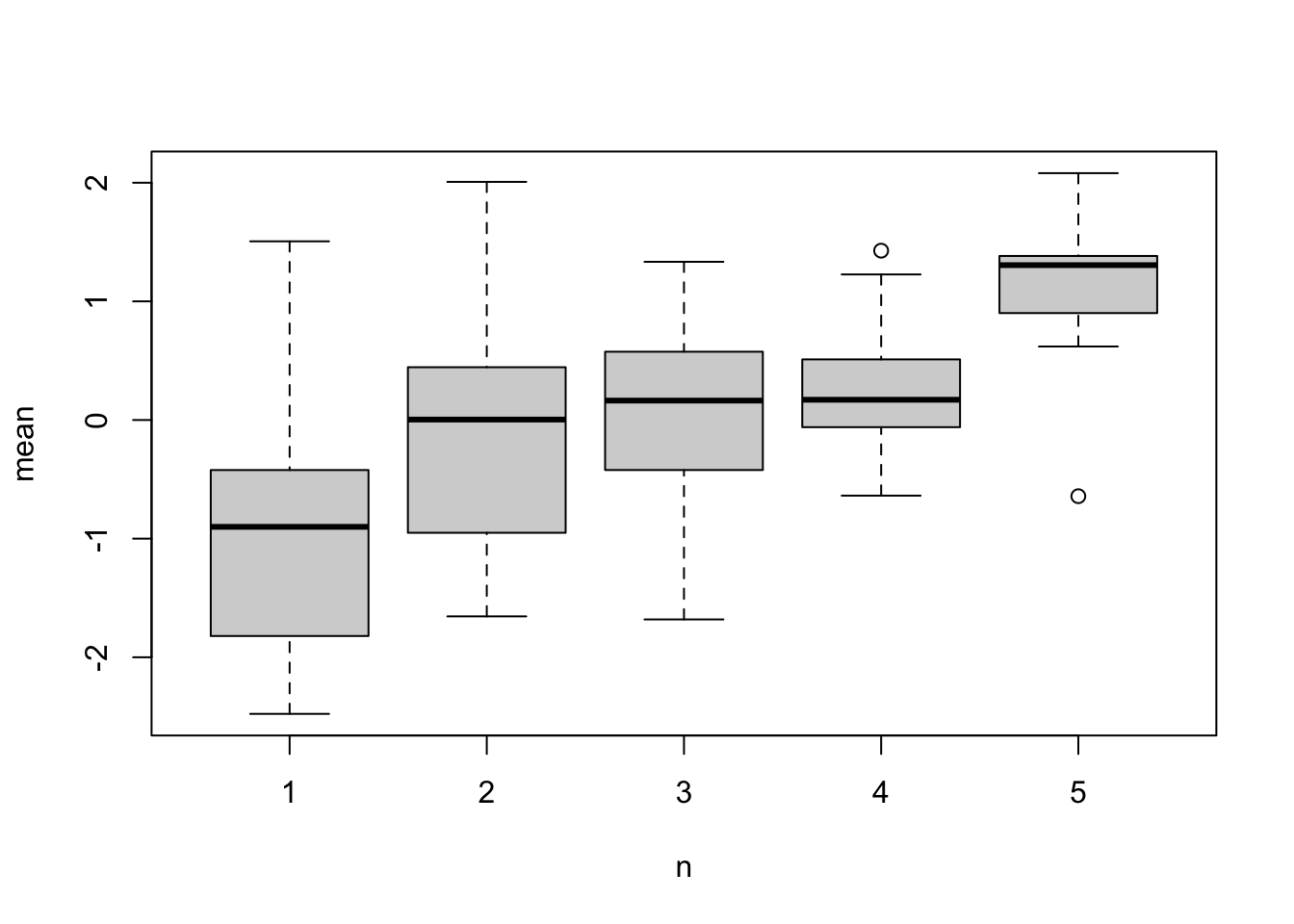
## [1] 262Lets try and visualise this. We know there is lots f between individual variation, and we know sampling is based on phenotype, so we would expect an association between number of observations and phenotype:
ind_data <- data.frame(
  n=as.vector(table(sample_data$individual)),
  mean=tapply(sample_data$y,sample_data$individual,mean)
  )
boxplot(mean~n,ind_data)