1.3 Interactions and non-linear effects

1.3.1 Interactions

\[ y_i = \beta_0 + \beta_1 x_{1i} + \beta_2 x_{2i} + \beta_3 x_{1i}x_{2i} + \epsilon_i \]

We can specify the interaction between two predictors by adding an interactions list to the parameters list. Interactions can then be specified between two named variables using “:”. Interactions can be specified between two predictors at the same level, or at different hierarchical levels.

squid_data <- simulate_population(
  n=2000,
  response_name = "body_mass",
  parameters=list(
    observation=list(
      names=c("temperature","rainfall"),
      beta = c(0.5,0.3)
    ),
    residual=list(
      vcov=0.3
    ),
    interactions=list(
      names=c("temperature:rainfall"),
      beta = c(-0.1)
    )
  )
)

data <- get_population_data(squid_data)
head(data)

##    body_mass temperature   rainfall   residual temperature:rainfall squid_pop
## 1 -0.1950863   0.6545190  1.5577734 -0.8877186            1.0195922         1
## 2 -0.8352969  -1.3405423  0.3989025 -0.3381711           -0.5347457         1
## 3 -0.2615434  -1.2677241 -0.2484353  0.4783440            0.3149474         1
## 4  0.8427175   0.8669511  0.1360867  0.3802140            0.1179805         1
## 5 -0.8451921  -1.8557505  0.8777406 -0.3435258           -1.6288676         1
## 6  0.7969244  -0.2192104  0.8250010  0.6409444           -0.1808488         1

coef(lm(body_mass ~ temperature * rainfall, data))

##          (Intercept)          temperature             rainfall 
##          0.006055206          0.487910683          0.284464667 
## temperature:rainfall 
##         -0.084342268

1.3.2 Non-linear effects

Polynomial (quadratic, cubic, etc) functions are essentially interactions with the same predictor. They can therefore be specified in the same way:

squid_data <- simulate_population(
  n=2000,
  response_name = "body_mass",
  parameters=list(
    observation=list(
      names=c("temperature"),
      beta = c(0.5)
    ),
    interactions=list(
      names=c("temperature:temperature"),
      beta = c(-0.3)
    ),
    residual=list(
      vcov=0.3
    )
  )
)
data <- get_population_data(squid_data)

plot(body_mass ~ temperature, data, pch=19, cex=0.5, col=alpha(1,0.5))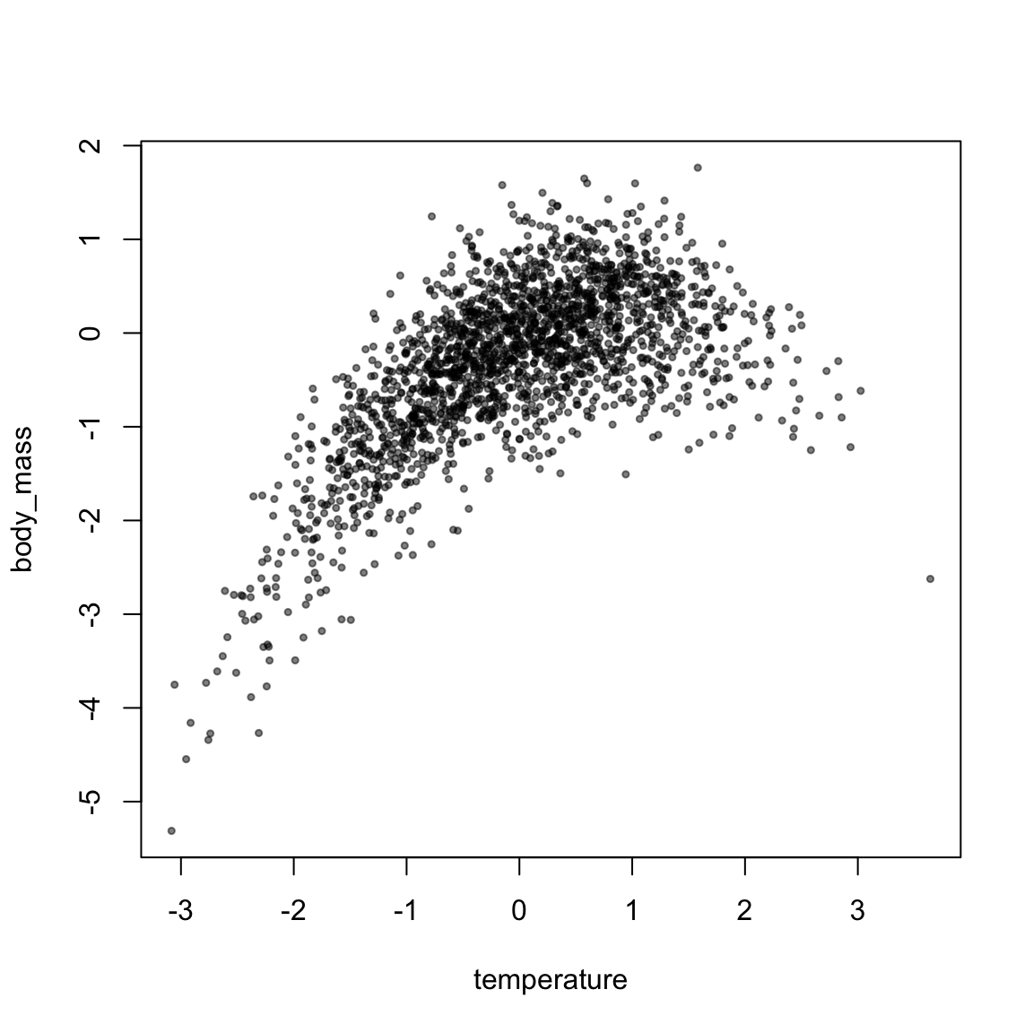

coef(lm(body_mass ~ temperature + I(temperature^2), data))

##      (Intercept)      temperature I(temperature^2) 
##     -0.003753765      0.510987516     -0.299719778