1.5 Known Predictors

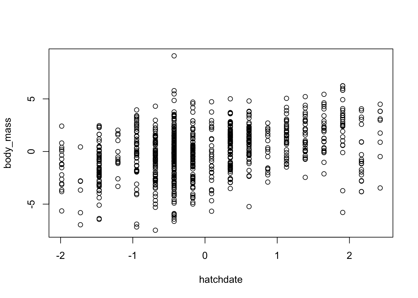
We might want to use existing predictors, rather than simulated ones, in our simulations. This has the advantage that any quirks of existing data (like a strange distribution) can be maintained. These predictors can be fed into the simulate_population() function, using the known_predictors argument. This argument takes a list, with one item, called predictors, a matrix or dataframe of predictors and one item called beta, a vector with the beta values for the respective predictors. Importantly, the predictors have to be the same length as number of observations in the simulated data. We can demonstrate this using the blue tit data set that comes with the MCMCglmm package.

library(MCMCglmm)
data(BTdata)

head(BTdata)

##        tarsus       back  animal     dam fosternest  hatchdate  sex
## 1 -1.89229718  1.1464212 R187142 R187557      F2102 -0.6874021  Fem
## 2  1.13610981 -0.7596521 R187154 R187559      F1902 -0.6874021 Male
## 3  0.98468946  0.1449373 R187341 R187568       A602 -0.4279814 Male
## 4  0.37900806  0.2555847 R046169 R187518      A1302 -1.4656641 Male
## 5 -0.07525299 -0.3006992 R046161 R187528      A2602 -1.4656641  Fem
## 6 -1.13519543  1.5577219 R187409 R187945      C2302  0.3502805  Fem

We can see that in this dataset there are several continuous predictors. Here we will use “hatchdate” and “tarsus”.

squid_data <- simulate_population(
  n = nrow(BTdata),
  response_name = "body_mass",
  parameters = list(
    observation =list(
      names = c("temperature","rainfall"),
      beta = c(0.5,0.3)
    ),
    residual = list(
      vcov = 0.3
    )
  ),
  known_predictors = list(
    predictors = BTdata[,c("hatchdate","tarsus")], 
    beta = c(1,2))
)

data <- get_population_data(squid_data)
head(data)

##   body_mass temperature     rainfall     residual  hatchdate      tarsus
## 1 -4.286821   0.5290832  0.375800507 -0.192105859 -0.6874021 -1.89229718
## 2  1.858944   0.3625056  0.002274996  0.092191340 -0.6874021  1.13610981
## 3  1.638961  -0.1032856  0.492434356  0.001475751 -0.4279814  0.98468946
## 4 -1.182909   0.3381428  1.479198475 -1.088091557 -1.4656641  0.37900806
## 5 -3.318436  -2.4582996 -0.693746732 -0.264992183 -1.4656641 -0.07525299
## 6 -1.858113   1.6906011 -0.309655352 -0.690406667  0.3502805 -1.13519543
##   squid_pop
## 1         1
## 2         1
## 3         1
## 4         1
## 5         1
## 6         1

plot(body_mass~hatchdate,data)