4.3 Sex specific genetic variance and inter-sexual genetic correlations

ds <- data.frame(animal=gryphons[,"id"],sex=sample(c("Female","Male"),nrow(gryphons), replace=TRUE))

squid_data <- simulate_population(
  parameters = list(
    sex=list(
      fixed=TRUE,
      names=c("Female","Male"),
      beta=c(-0.5,0.5)
    ),
    animal= list(
      names = c("G_female","G_male"),
      vcov =matrix(c(0.1,-0.1,-0.1,0.4), nrow=2, ncol=2 ,byrow=TRUE)
      ),
    residual = list(
      names="residual",
      vcov = 0.1
    )
  ),
  data_structure = ds,
  pedigree = list(animal=ped),
  model = "y = Female + Male + I(Female)*G_female + I(Male)*G_male + residual"
)

data <- get_population_data(squid_data)
head(data)

##            y Female Male    G_female     G_male    residual animal    sex
## 1 -1.1406269      1    0 -0.41650798  0.8611695 -0.22411895    204 Female
## 2 -0.9338681      1    0  0.02895999  0.7161771 -0.46282805    205 Female
## 3 -0.5726704      1    0 -0.11908647  0.3606215  0.04641609    206 Female
## 4  0.5511020      0    1 -0.45076138  0.2253053 -0.17420333    207   Male
## 5 -0.6838055      1    0 -0.12133713 -0.3310633 -0.06246839    208 Female
## 6 -0.1827386      0    1  0.33321284 -0.6581778 -0.02456084    209   Male
##   squid_pop
## 1         1
## 2         1
## 3         1
## 4         1
## 5         1
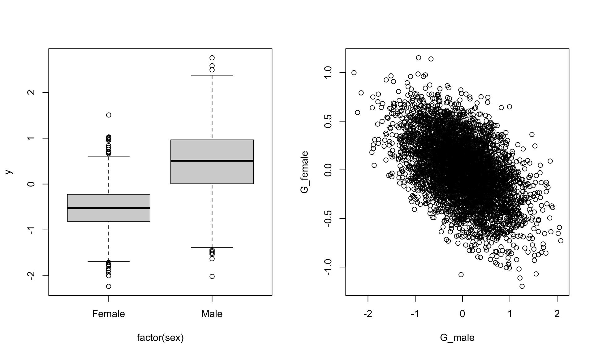
## 6         1

par(mfrow=c(1,2))
boxplot(y~factor(sex),data)
plot(G_female~G_male,data)