6.4 Spatial Autocorrelation

Spatial autocorrelation can be simulate by passing a spatial correlation matrix to the cov_str argument of simulate_population().

First we need some kind of spatial autocorrelation matrix. This is a large correlation matrix, showing how close all the locations are to each other. We create different kinds of these. Here, we use the corClasses structures in the nlme package. To demonstrate, we generate a exponential spatial correlation matrix, with strong autocorrelation.

library(nlme)

## 
## Attaching package: 'nlme'

## The following object is masked from 'package:lme4':
## 
##     lmList

## The following object is masked from 'package:dplyr':
## 
##     collapse

library(squidSim)

ds <- make_structure("location(2500)")
locations <- matrix(1:2500,nrow=50,ncol=50)
locations2<-as.data.frame(t(sapply(1:2500,function(x)which(locations==x, arr.ind=TRUE))))
colnames(locations2) <- c("x","y")

cs1Exp <- corExp(5, form = ~ x + y)
cs1Exp <- Initialize(cs1Exp, locations2)
spM<- corMatrix(cs1Exp)
colnames(spM) <- rownames(spM) <- 1:2500

We can feed this matrix into the cor_str argument of simulate_population(). Here we simulate with and without spatial autocorrelation to show the difference.

sim_dat_auto<-simulate_population(
  seed=22,
  data_structure = ds,
  parameters = list(
    location = list(vcov=4),
    residual = list(vcov=1)
  ),
  cov_str = list(location=spM)
)
dat_auto<-get_population_data(sim_dat_auto)


sim_dat_no<-simulate_population(
  seed=27,
  data_structure = ds,
  parameters = list(
    location = list(vcov=4),
    residual = list(vcov=1)
  )
)
dat_no<-get_population_data(sim_dat_no)

library(viridis)

## Loading required package: viridisLite

## 
## Attaching package: 'viridis'

## The following object is masked from 'package:scales':
## 
##     viridis_pal

color_scale <- viridis(20)

dat_auto$y_group <- as.numeric(cut(dat_auto$y, breaks=20))
dat_no$y_group <- as.numeric(cut(dat_no$y, breaks=20))

par(mfrow=c(1,2))
plot(y~x,locations2, pch=19, col=color_scale[dat_auto$y_group], cex=1, main="Spatial Autocorrelation")
plot(y~x,locations2, pch=19, col=color_scale[dat_no$y_group], cex=1, main="No Autocorrelation")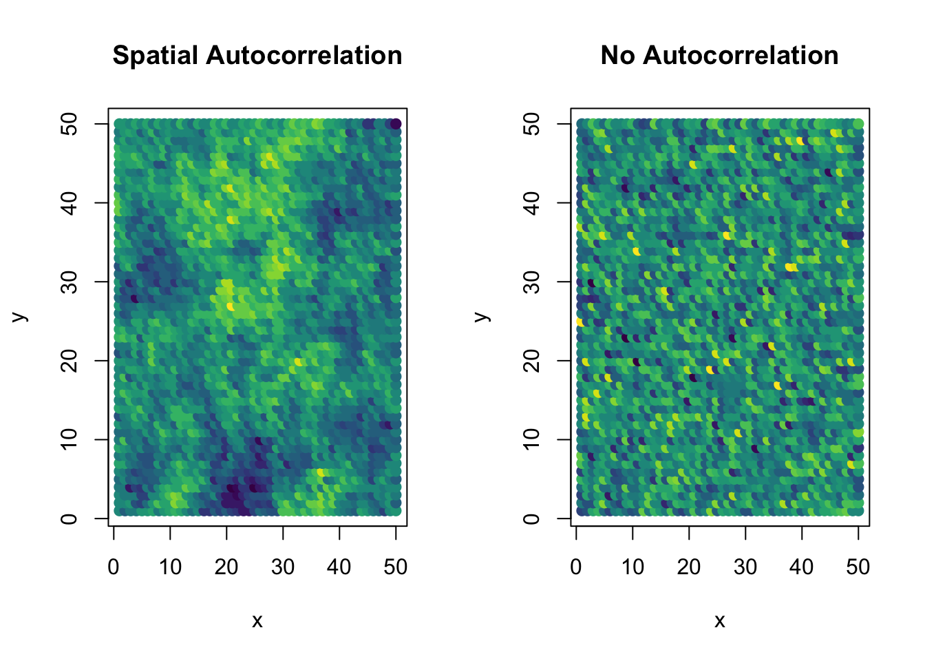

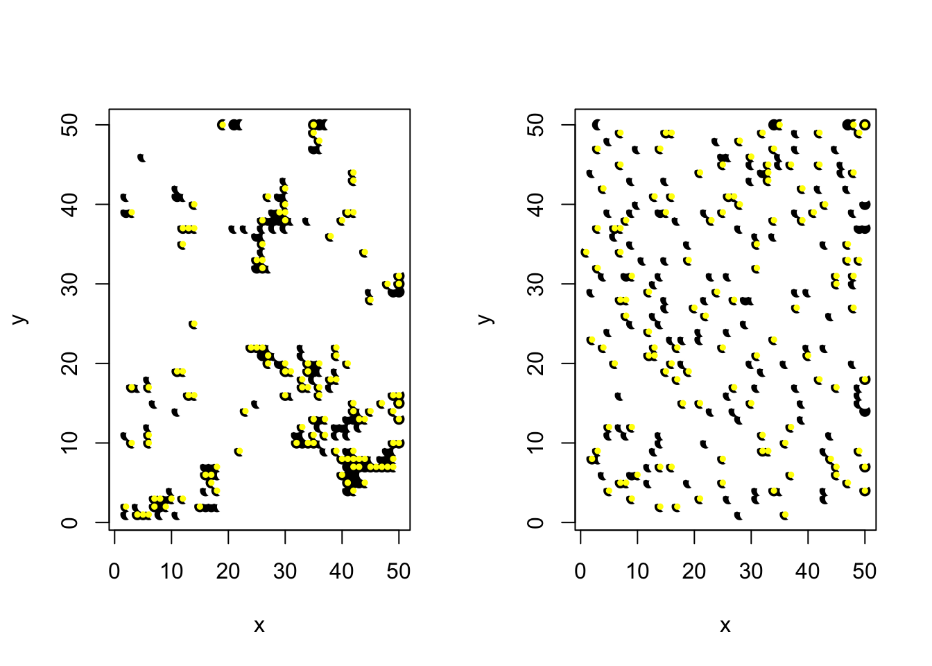
6.4.1 Example: Species occurrence data with spatial autocorrelation

library(nlme)
library(squidSim)

ds <- make_structure("location(2500)")
locations <- matrix(1:2500,nrow=50,ncol=50)
locations2<-as.data.frame(t(sapply(1:2500,function(x)which(locations==x, arr.ind=TRUE))))
colnames(locations2) <- c("x","y")

cs1Exp <- corExp(3, form = ~ x + y)
cs1Exp <- Initialize(cs1Exp, locations2)
spM<- corMatrix(cs1Exp)
colnames(spM) <- rownames(spM) <- 1:2500

sim_dat<-simulate_population(
  seed=236,
  data_structure = ds,
  n_response=2,
  response_names = c("occurrence","observation"),
  parameters = list(
    intercept= c(-3,0),
    location = list(vcov=c(4,0)),
    # age=list(covariate=TRUE,  beta=matrix(c(-0.2,0),ncol=2)),
    residual=list(vcov=c(0,0))
  ),
  cov_str = list(location=spM),
  family= "binomial",
  link="probit"
)
dat<-get_population_data(sim_dat)
dat$seen <- dat$occurrence* dat$observation



sim_dat_R<-simulate_population(
  seed=224,
  data_structure = ds,
  n_response=2,
  response_names = c("occurrence","observation"),
  parameters = list(
    intercept= c(-3,0),
    residual=list(vcov=c(4,0))
  ),
  family= "binomial",
  link="probit"
)
dat_R<-get_population_data(sim_dat_R)
dat_R$seen <- dat_R$occurrence* dat_R$observation

par(mfrow=c(1,2))
plot(y~x,locations2, pch=19, col=dat$occurrence)
points(y~x,locations2[dat$seen==1,], pch=19, col="yellow", cex=0.5)

plot(y~x,locations2, pch=19, col=dat_R$occurrence)
points(y~x,locations2[dat_R$seen==1,], pch=19, col="yellow", cex=0.5)