6.1 Simple Temporal Effects
We might have measured a variable over the course of a certain time period (e.g. 20 years). We might expect that there is stochastic year-to-year variation, which we can simulate already. However we might also want to simulate patterns in that temporal data. We can treat the levels associated with a particular grouping factor (e.g. year) as both a factor and continuous.
To treat a grouping factor as continuous, we use covariate=TRUE in the parameter list. In this way we can simulate a linear effect of year:
squid_data <- simulate_population(
  data_structure= make_structure(structure = "year(20) + sex(2)/individual(50)",repeat_obs=20),
  parameters=list(
    year_cont = list(
      group="year",
      names= "year_cont",
      covariate=TRUE,
      beta=0.3
    ),
    year = list(
      vcov = 0.8
    ),
    residual=list(
      vcov = 1
      )
    )
)
note we have specified group in the parameter list. This enables us to link a set of parameters to the grouping factor in the data structure. This doesn’t have to be specified and defaults to the name of the list item.
data <- get_population_data(squid_data)
head(data)
## y year_cont year_effect residual year sex individual squid_pop
## 1 1.1436403 1 2.21821 -1.3745698 1 1 1 1
## 2 3.0559676 1 2.21821 0.5377575 1 1 1 1
## 3 4.2148492 1 2.21821 1.6966392 1 1 1 1
## 4 0.6152528 1 2.21821 -1.9029573 1 1 1 1
## 5 1.8172122 1 2.21821 -0.7009978 1 1 1 1
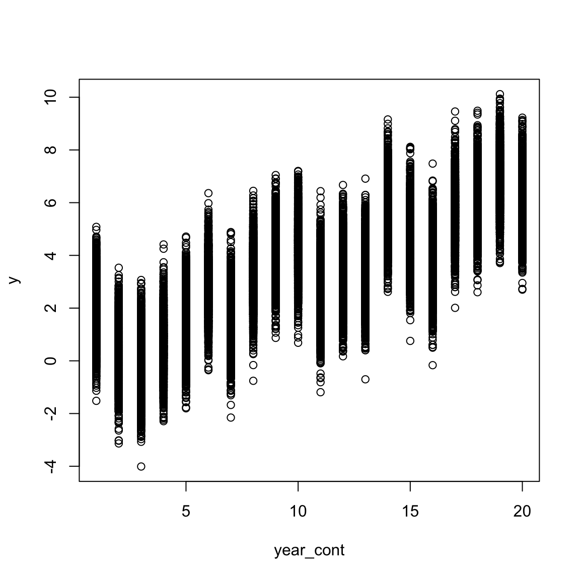
## 6 1.7139274 1 2.21821 -0.8042827 1 1 1 1plot(y ~ year_cont, data)
Here we can see there is within year variation, year to year variation, as well as a linear directional year effect.
lmer(y ~ year_cont + (1|year), data)## Linear mixed model fit by REML ['lmerMod']
## Formula: y ~ year_cont + (1 | year)
## Data: data
## REML criterion at convergence: 113318.3
## Random effects:
## Groups Name Std.Dev.
## year (Intercept) 0.9652
## Residual 0.9956
## Number of obs: 40000, groups: year, 20
## Fixed Effects:
## (Intercept) year_cont
## 0.5669 0.2838In a similar way we can also simulate a quadratic effect of time.
squid_data <- simulate_population(
  data_structure = make_structure(structure = "year(20) + sex(2)/individual(50)",repeat_obs=20),
  parameters=list(
    year_cont = list(
      group="year",
      names= c("year_cont"),
      covariate=TRUE,
      beta=c(0.3)
    ),
    interactions=list(
      names= c("year_cont:year_cont"),
      beta=c(-0.05)
    ),
    year = list(
      vcov = 1
    ),
    residual=list(
      vcov = 0.8
    )
  )
)

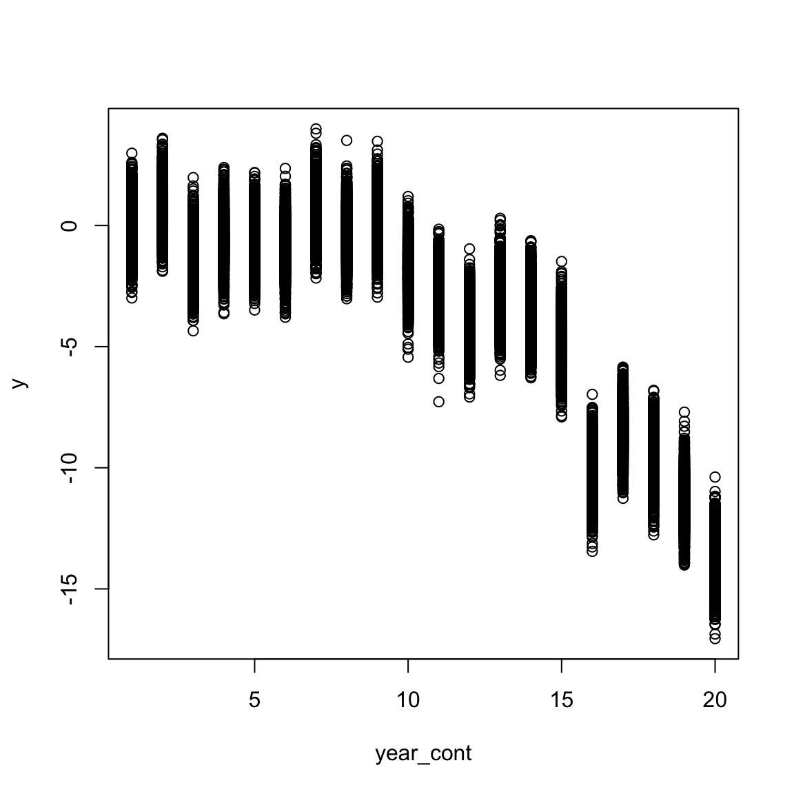
data <- get_population_data(squid_data)

plot(y~year_cont,data)