2.2 Factors
In the first sections, we just simulated continuous predictors, varying at the level of the observation. However, we may want to simulate factors with known or fixed effects (i.e. not variables drawn randomly from a particular distribution) at different levels, such as sex or treatment effects.
The first thing we want to do is specify a simple data structure, for example 100 observations for each of two sexes:
ds <- make_structure(structure="sex(2)", repeat_obs=100, level_names=list(sex=c("female","male")))Then we feed this data structure into the simulate_population() function using the data_structure argument. Note that we no longer need to specify the sample size (n), as this is taken from the number of rows in the data_structure.
squid_data <- simulate_population(
  data_structure = ds,
  parameters = ...
)
In order to tell the parameter list we have effects that vary at different hierarchical levels, we can create additional slots in the parameter list for the grouping factors, so now it will look something like:
squid_data <- simulate_population(
  data_structure = ds,
  parameters = list(
    intercept = ...,
    sex = list(
      ...
    ),
    observation = list(
      ...
    ),
    residual = list(
      ...
    )
  )
)
The names in the parameter list that relate to the different grouping factors either need to match the name in the data structure exactly (as above) or a ‘group’ argument needs to be given e.g.
squid_data <- simulate_population(
  data_structure = ds,
  parameters = list(
    intercept = ...,
    anything = list(
      group="sex,"
      ...
    ),
    observation = list(
      ...
    ),
    residual = list(
      ...
    )
  )
)
We then need to tell the parameters list that we have fixed effects for this grouping factor, in other words we know the difference in body size between the sexes is 0.5, for example. To do this we specify fixed = TRUE.
squid_data <- simulate_population(
  data_structure = ds,
  parameters = list(
    intercept = ...,
    sex = list(
      fixed=TRUE,
      ...
    ),
    observation = list(
      ...
    ),
    residual = list(
      ...
    )
  )
)
We can then give a beta for all the different levels of that group. Note that there are two ways to specify this, as there also is in linear models in R. First, we can specify an intercept, and contrasts, equivalent to the output of lm(body_mass~sex), which involves specifying the beta for the first level as 0 to make it the baseline level (or any other level that you would like to be the baseline). Note that, as of version 0.2.4, if the levels for this grouping factor in the data structure have names (in this case “male” and “female”), then the same names have to be specified in the parameter list.
squid_data <- simulate_population(
  data_structure = ds,
  parameters = list(
    intercept= 10,
    sex=list(
      fixed=TRUE,
      beta=c(0,0.5),
      names = c("female","male")
    ),
    residual = list(
      vcov = 0.5
    )
  )
)

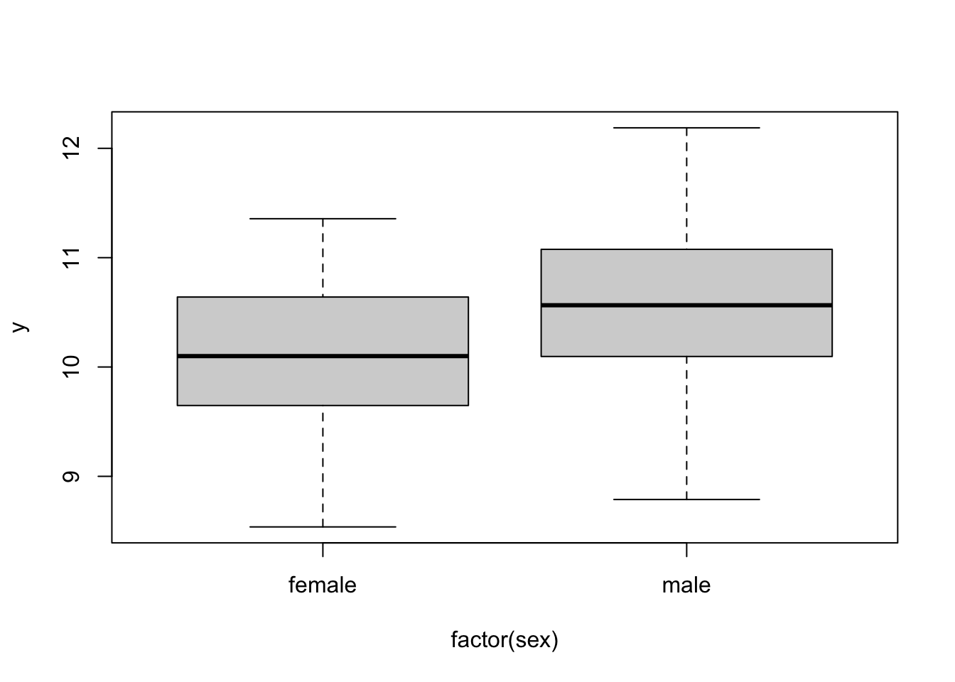
data <- get_population_data(squid_data)

boxplot( y ~ factor(sex), data)
lm( y ~ factor(sex), data)##
## Call:
## lm(formula = y ~ factor(sex), data = data)
##
## Coefficients:
## (Intercept) factor(sex)male
## 10.176 0.377Alternately, we can specify no intercept (which defaults to 0), and the means for the two levels as betas (equivalent to lm(body_mass~0+sex)):
squid_data <- simulate_population(
  data_structure = ds,
  parameters = list(
    sex=list(
      fixed=TRUE,
      beta=c(10,10.5),
      names = c("female","male")
    ),
    residual = list(
      vcov = 0.5
    )
  )
)

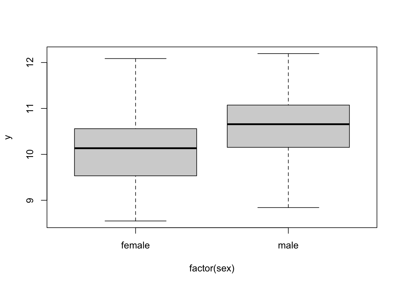
data <- get_population_data(squid_data)

boxplot( y ~ factor(sex), data)
lm( y ~ factor(sex), data)##
## Call:
## lm(formula = y ~ factor(sex), data = data)
##
## Coefficients:
## (Intercept) factor(sex)male
## 10.132 0.409lm( y ~ 0+factor(sex), data)##
## Call:
## lm(formula = y ~ 0 + factor(sex), data = data)
##
## Coefficients:
## factor(sex)female factor(sex)male
## 10.13 10.54We would recommend the former method, as this makes things clearer if other factors are simulated.
2.2.1 Fixed Factor Interactions
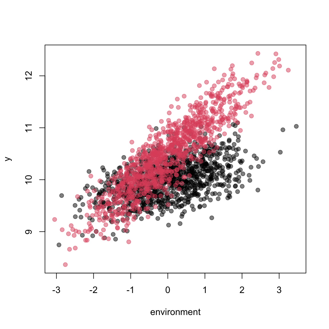
We might want to simulate an interaction between a continuous predictor and a factor, for example the effect of the environment varying between two sexes. Specifying this using simulate_population() is similar to interactions between two continuous predictors that we have previously encountered (Section 1.3). In the interaction part of the parameter list, we now specify the contrasts between the slopes for environment, using the names that we have assigned the different levels. In the simulation below, males are larger, and have a larger environment slope:
squid_data <- simulate_population(
  data_structure = make_structure(structure = "sex(2)", repeat_obs=1000),
  parameters = list(
    intercept=10,
    sex=list(
      fixed=TRUE,
      names=c("female","male"),
      beta=c(0,0.5)
    ),
    observation= list(
      names = c("environment"),
      beta =c(0.2)
      ),
    interactions = list(
      names=c("environment:male"),
      beta = 0.4
      ),
    residual = list(
      names="residual",
      vcov = 0.1
    )
  )
)

data <- get_population_data(squid_data)
head(data)
## y female male environment residual environment:male sex squid_pop
## 1 9.750474 1 0 -1.25796735 0.002067288 0 1 1
## 2 10.456740 1 0 -0.92214063 0.641167781 0 1 1
## 3 10.327966 1 0 0.67783250 0.192399695 0 1 1
## 4 9.976236 1 0 0.71095086 -0.165954375 0 1 1
## 5 9.984801 1 0 -0.08647446 0.002095792 0 1 1
## 6 10.295880 1 0 2.87982801 -0.280085298 0 1 1plot(y~environment,data, pch=19, col=scales::alpha(c(1,2),0.5)[factor(data$sex)])
lm( y ~ 0 + factor(sex)*environment, data)##
## Call:
## lm(formula = y ~ 0 + factor(sex) * environment, data = data)
##
## Coefficients:
## factor(sex)1 factor(sex)2 environment
## 10.0031 10.4872 0.2023
## factor(sex)2:environment
## 0.3867