1.2 Correlated predictors

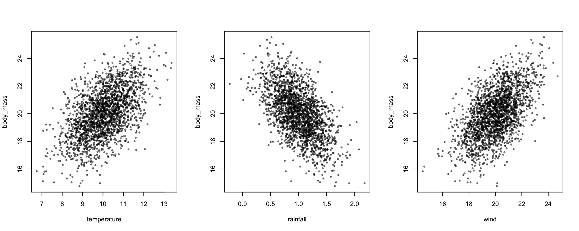
We can also simulate correlations between these predictors, as vcov specifies the variance/covariance matrix of the predictors.

squid_data <- simulate_population(
  n=2000,
  response_name = "body_mass",
  parameters=list(
    intercept=10,
    observation=list(
      names=c("temperature","rainfall", "wind"),
      mean = c(10,1 ,20),
      vcov =matrix(c(
        1, 0, 1,
        0,0.1,0,
        1, 0, 2
        ), nrow=3 ,ncol=3,byrow=TRUE),
      beta =c(0.5,-3,0.4)
    ),
    residual=list(
      vcov=1
    )
  )
)

data <- get_population_data(squid_data)

library(scales)
par(mfrow=c(1,3))
plot(body_mass ~ temperature + rainfall + wind, data, pch=19, cex=0.5, col=alpha(1,0.5))

coef(lm(body_mass ~ temperature + rainfall + wind, data))

## (Intercept) temperature    rainfall        wind 
##   9.7745865   0.4847876  -2.9889811   0.4172907

Matrices in R

To code a matrix in R we use the matrix function (see ?matrix). This takes a vector of values, and arranges then in a matrix, with dimensions specified with nrow and ncol. By default it fills the matrix by column, which can be changed to per row, by specifying byrow=TRUE. For big matrices this can be petty annoying. TheTri2M() function from the package MCMCglmm allows you to just give the lower or upper half of the matrix, and it will fill the rest out for you. For example, we can make a correlation matrix using:

Tri2M(c(1,0.5,1,0.3,0.2,1), lower.tri = FALSE, diag=TRUE)

##      [,1] [,2] [,3]
## [1,]  1.0  0.5  0.3
## [2,]  0.5  1.0  0.2
## [3,]  0.3  0.2  1.0

Instead of specifying a variance-covariance matrix (vcov), we can also specify a variance-correlation matrix (variance on the diagonals and correlations on the off-diagonals), using vcorr

squid_data <- simulate_population(
  n=2000,
  response_name = "body_mass",
  parameters=list(
    intercept=10,
    observation=list(
      names=c("temperature","rainfall", "wind"),
      mean = c(10,1,20),
      vcorr =matrix(c(
         1,  -0.2, 0.5,
       -0.2,  0.1, 0.3,
        0.5,  0.3,  2
        ), nrow=3 ,ncol=3,byrow=TRUE),
      beta =c(0.5,-3,0.4)
    ),
    residual=list(
      vcov=1
    )
  )
)

data <- get_population_data(squid_data)

cor(data[,c("temperature","rainfall", "wind")])

##             temperature   rainfall      wind
## temperature   1.0000000 -0.1812635 0.5176010
## rainfall     -0.1812635  1.0000000 0.2617843
## wind          0.5176010  0.2617843 1.0000000

Through simulating correlated predictors, we can also simulate more interesting phenomena. For example, we may want to simulate the effect of a correlated missing predictor. Here, rain and wind, but not temperature, affect adult body mass, but only temperature and rainfall are measured:

squid_data <- simulate_population(
  n=2000,
  response_name = "body_mass",
  parameters=list(
    intercept=10,
    observation=list(
      names=c("temperature","rainfall", "wind"),
      mean = c(10,1 ,20),
      vcov =matrix(c(
        1, 0, 1,
        0,0.1,0,
        1, 0, 2
        ), nrow=3 ,ncol=3,byrow=TRUE),
      beta =c(0.5,-3,0.4)
    ),
    residual=list(
      vcov=1
    )
  )
)

data <- get_population_data(squid_data)

library(scales)
par(mfrow=c(1,3))
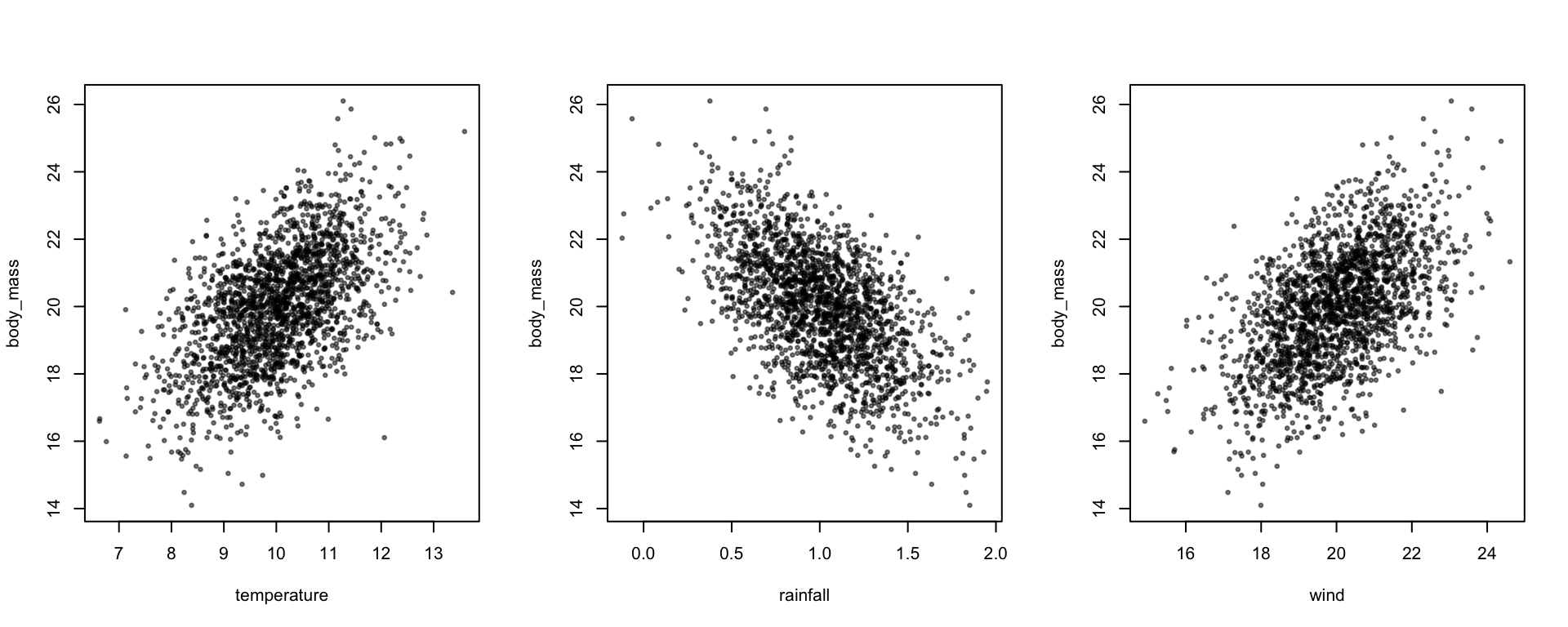
plot(body_mass ~ temperature + rainfall + wind, data, pch=19, cex=0.5, col=alpha(1,0.5))

coef(lm(body_mass ~ temperature + rainfall, data))

## (Intercept) temperature    rainfall 
##  13.8936511   0.9148843  -3.0592937

coef(lm(body_mass ~ temperature + rainfall + wind, data))

## (Intercept) temperature    rainfall        wind 
##  10.2631334   0.5509808  -3.0467600   0.3633353

We can also use this to induce measurement error in a predictor - we can simulate the true variable with a certain effect on the response, and another correlated variable - the measured variable - with no direct effect on the response. The correlation between these two variables represents the measurement error (the repeatability of the variable is the correlation squared).